NWP SAF: Bias correction procedures for ATOVS

Bias Correction of (A)TOVS Radiances

Richard Renshaw, Met Office

Please note, we are currently reviewing the content of this guide as it has not been updated for some years and no longer reflects the current status at the Met Office.
However, you may still find useful information on the general principles, and some specific methods, of satellite radiance bias correction.

Contents:

Introduction
Current scheme
Other schemes
Choice of reference
Diurnal effects
Scan dependence
Surface dependence
Time dependence
Choice of predictors
References

Introduction

bias in the NWP background fields
errors in the forward process, for instance in the radiative transfer
residual contamination of the observations from cloud or other sources
instrument calibration errors
inaccurate specification of instrument spectral response filters

Bias also varies with scan angle:

Note that all recommendations are based on experience at the Met Office and may not be the best choice for all centres.

Current scheme

Eyre (1992)

Scan-dependent corrections are calculated as mean values of O-B for each scan position.
Residual bias is modelled as the sum of an offset term plus coefficient times each of several predictors. For TOVS we use observed brightness temperature in MSU channels 2,3,4 as predictors. For ATOVS we use AMSU channels 5 and 9. These predictors define in some sense the airmass, and the residual bias is modelled as being a function of airmass. We use just one set of coefficients and offset, for all scan positions, latitudes and surface types.
The values are recalculated monthly. The offset and coefficients are calculated from the previous month's data by linear regression. Often we decide not to change the current operational corrections if we see no problems with the current set.

Deficiencies of current scheme

Use of data over high land
The lowest microwave predictors (MSU 2 and AMSU 5) see little of the surface when the surface is near sea level. As elevation increases they see more and more of the surface. Over areas of high land it is no longer appropriate to use them as predictors in the same way as over sea. We therefore use no TOVS or ATOVS data where the surface height is over 1km. This plot shows spots rejected by 1D-Var in a six-hour period. Those coloured black are rejected on the basis of surface height. Many areas are affected, including Antarctica, Greenland, and the Tibetan plateau.
Residual scan-dependent bias
The scheme was originally applied to limb-corrected data. The scan-dependent correction removed scan-dependent bias, and the airmass-dependent correction had little variation with scan position. We now use data with no limb-correction applied. The microwave brightness temperatures we use as predictors vary across the scan, and so the airmass-dependent correction will also vary. The following shows HIRS channel 12 mean O-B before bias correction (solid line), after scan-dependent correction (dotted line), and after full bias correction (dashed line). The airmass correction has introduced a scan-dependent bias. Data is from April 2000 and the corrections were those used operationally at that time, calculated from December 1999 data.
Use over land
Bias corrections are calculated from spots over sea and sea-ice only, but the corrections are used globally. Below are mean values for the two ATOVS predictors, AMSU channels 5 and 9, for June 1999. The predictors take extreme values over Antarctica, outside the range of values encountered by the linear regression. Channel 5 takes extreme values over land areas in the Tropics, not all high land.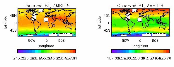

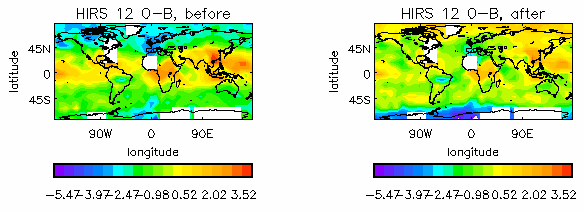
The following shows mean O-B for HIRS 12 from this period, before and after bias correction. Correction coefficients for this channel are 0.044 x AMSU 5 and -0.188 x AMSU 9. At extreme latitudes the correction scheme is not removing the bias successfully.

Other schemes

Variational bias correction

Fixed scan-dependent correction. A single mean value is calculated for each channel, each scan position.
Residual from (i) is modelled as an airmass-dependent correction with a predictor which is lapse rate convolved with weighting function.
Any remaining bias is treated by a time-dependent component consisting of an airmass-dependent correction with predictors lower tropospheric lapse rate, upper tropospheric lapse rate, squares of these lapse rates, local zenith angle, and an offset.

The 'lapse rate convolved with weighting function' predictor is designed to solve a specific problem. Errors in the spectroscopy or in the instrument response function may lead to errors in the height of the weighting function as calculated by the radiative transfer model. If the atmosphere were isothermal, and so lapse rate was zero, then such errors would have no effect. When the atmosphere is not isothermal, the effect of such an error on the calculated brightness temperature can be approximated as a constant times this predictor. Strictly the predictor should include a surface term -d(Brightness Temperature)/d(Surface Pressure) to allow for the observation seeing more or less of the surface than estimated by the RT model. This may be particularly important for channels such as AMSU 4 where sensitivity to the surface is very much a function of scan angle.

Harris and Kelly scheme

Eyre

Harris and Kelly (2001)

ECMWF calculate bias corrections relative to the NWP model background but are careful to use only data close to radiosonde stations. The corrections are calculated as follows:

scan-dependent correction
The scan-dependent correction is calculated individually for 10 degree latitude bands. Northernmost and southernmost bands are broadened to give a reasonable capture of data. The correction is then smoothed between latitude bands to give a smooth transition across the band boundaries.
airmass-dependent correction
The residual is modelled as a function of the following predictors taken from the NWP model background:
- 1000-300hPa thickness
- 200-50hPa thickness
- surface skin temperature (SST)
- total column water vapour

Coefficients are calculated globally, not by latitude band. Some weighting is applied in the regression to ensure for instance that stratospheric channels are not dependent on the SST predictor. Harris and Kelly show that surface skin temperature is particularly useful in modelling biases which change between sea and sea-ice. ECMWF update the bias corrections when there are major updates to their NWP system but otherwise try to keep them fixed.

Choice of reference

satellite-measured radiances
AMSU is considered to be a well-calibrated instrument and so a potential choice of reference. McNally (ECMWF, pers comm) has experimented with applying no bias correction to certain AMSU channels. Impact on forecast skill was negative.
NWP model background
Data is available globally, a distinct advantage. There are known to be biases both in the NWP data and in the radiative transfer models required to calculate radiances. In practice it has not proved possible to distinguish between the various sources of bias, and so the bias corrections calculated include corrections for deficiencies in NWP.
NWP model analysis
The NWP background is a 6-hour forecast, during which time the model has "spun up" from the previous analysis. The latest analysis will have the benefit of the latest observations. Plots of mean (Analysis-Background) temperatures at 850hPa and 500hPa from tests of the 1999 "Autumn Package" show little large-scale bias. Differences are localised. This would suggest there is little advantage in using model analyses as reference instead of model background. Roger Saunders (pers. comm.) reports this has been tried at ECMWF, with little effect. Another consideration is the technical difficulty involved. Radiances calculated from the model background are available "for free" from OPS 1DVAR. They aren't currently calculated from model analyses.
colocated radiosonde reports
This data source is not free from bias. Bouttier et al (1999) describe bias corrections applied to sonde temperatures by ECMWF; up to 4K for certain sonde types. The bias is related to solar radiation and so will have a seasonal component. Data coverage is also a problem. The oceans are poorly sampled, as are many land areas subject to extreme conditions, such as the Poles and Siberia. Even where coverage is good, the number of satellite observations colocated in time and space is limited.
model fields near radiosonde stations
This would require some work to implement. The only advantage over using colocated radiosonde reports is that the time and distance separation criteria (between sonde and radiance observation) can be relaxed. The model is effectively being used to interpolate. Otherwise, the same disadvantages apply.

Recommendation

Diurnal effects

In an attempt to measure this variation, mean O-B values were calculated separately for data from each of the global model run times (00Z,06Z,12Z,18Z, each +/- 3hrs). Means were calculated over a whole month (June 1999). Data coverage provides good overlap for 00Z/12Z and for 06Z/18Z data times. Below are mean 00Z values minus mean 12Z values, and mean 06Z minus 18Z values, for HIRS channel 8:

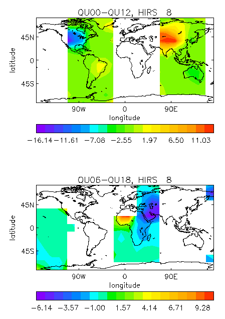
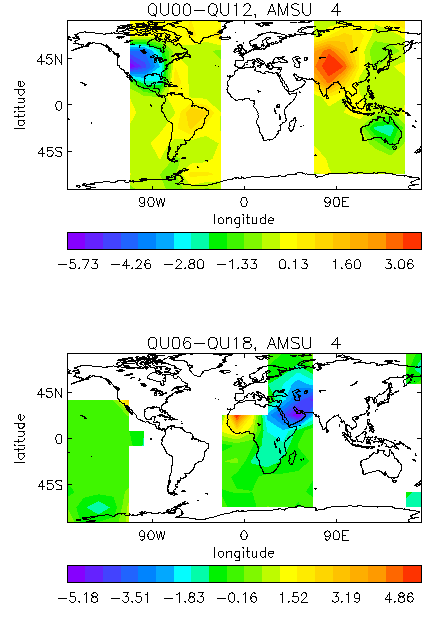
There are large differences over N.America, the Middle East, and the Tibetan plateau. A similar signal is seen in AMSU channel 4:

Barwell and Bradbury (1994) investigated differences in O-B radiance for HIRS channel 7 comparing NOAA-11 data with NOAA-12. The equator crossing times for the two satellites differed by about 3 hours. They concluded that use of the nearest 6-hourly NWP background field, with no time interpolation, was producing large differences in regions with significant diurnal variation in skin temperature. As of March 2000 the background fields are interpolated in time. Equivalent statistics since that change have not been produced.

Recommendation: If, as seems likely, diurnal biases are model rather than observation-based, there would seem to be little point in devising bias corrections to take account of this effect.

Scan dependence

Bias correction schemes typically have two steps:

subtract the mean bias as a function of scan angle
model the residual bias using airmass-dependent predictors

Below are O-B biases for AMSU channel 9 (June 1999) by latitude band and scan position. The mean bias changes with latitude. That can be corrected by an airmass-dependent correction. The shape of the bias across the scan also changes with latitude. It may be possible to correct this with an airmass-dependent correction if the predictors used vary with scan angle.

ECMWF make their scan-dependent correction a function of latitude. A similar argument to the above can be applied here. The scan correction varies with latitude. The airmass predictors also vary with latitude. The two corrections should be calculated simultaneously. A related question arises. The residual bias in a latitude band is the deviation from the mean in that latitude band. It is not clear that airmass coefficients which successfully correct the residual in one latitude band would be appropriate to another latitude band. Perhaps airmass coefficients in the ECMWF scheme should be calculated individually for each latitude band.

The ECMWF scheme effectively makes the scan correction airmass-dependent, but doesn't revise the calculation of other parts of the bias correction to take account of that. A full treatment would calculate airmass coefficients (and offset) individually for each scan position. That has technical problems in the Met Office system. We would have to archive bias statistics files many times larger than at present. We would also have to ensure that coefficients varied smoothly across the scan.

Recommendation:

Use fixed corrections for each scan position. We have sufficient data that each scan position is well represented in the statistics. Noise from differences in data sampling between the scan positions is small, and so modelling the scan-dependence with trigonometric functions wouldn't give any advantage.
Calculate scan-dependent corrections simultaneously with airmass-dependent components.
Scan-dependent corrections should be global values, although possibly dependent on surface type.

7. Surface dependence

Below is plotted mean O-B for NOAA-16 AMSU channels 5 and 12, for 5 latitude bands, from March 2001. Solid line shows values over land, dotted line over sea, and dashed over sea-ice.

AMSU channel 5 shows land values changing with latitude, but sea values fairly constant. This suggests that variation in the land values is due to errors in assumed emissivity and skin temperature, rather than being a function of airmass.

We can use a new predictor to try to model errors in emissivity. If the assumed emissivity has a bias, then to a first approximation the corresponding bias in calculated top-of-atmosphere radiance is proportional to surface skin temperature times surface-to-space transmittance. Skin temperature times transmittance may then be a useful predictor over land and sea-ice. Over the sea, we use FASTEM (English 1999) to calculate emissivity as a function of view angle, surface windspeed and skin temperature. Resultant errors in emissivity are likely to vary with windspeed, which may be a more appropriate predictor. These predictors are assessed in Choice of predictors below.

8. Time dependence

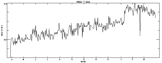
Below are global mean O-B values for AMSU channel 7, daily from April 1999 to March 2000. Day-to-day variations are generally small. On longer time-scales there are significant trends.

Below are correlations between AMSU channel 7 O-B and observed brightness temperatures in AMSU channels 5 (solid line), 7 (dotted) and 9 (dashed). These three channels were used as predictors at the Met Office, although now only channels 5 and 9 are used.

These correlations (together with cross-correlations between channels) determine the coefficients for the airmass-dependent correction. There would seem to be a seasonal cycle.

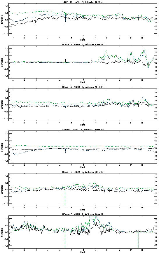
The correlations can be calculated as covariances for each latitude band normalised by global values of standard deviation. They give some idea of how consistently the predictors fit the variation of bias within each latitude band. There are noisy periods in the timeseries, in Winter and Spring for each hemisphere. This noise isn't apparent in the global timeseries.

Another feature to note is that these localised correlations are small, sometimes oscillating about zero. This suggests that the airmass-dependent correction is useful only in correcting biases on global scales. During the noisy periods correlations are sometimes high but rapidly changing. The fact that correlations are more noisy in the Southern Hemisphere than in the Northern suggests much of the variation is due to model errors.

9. Choice of predictors

Recent problems with individual instruments and with single channels on some instruments make the idea of using one channel as a predictor for the bias correction in another channel not so attractive. The following are considered here as candidate predictors for each channel:

850-300hPa temperature difference
200-50hPa temperature difference
NCEP use similar predictors. The choice of 850hPa avoids the need to extrapolate temperature below the surface for much of the globe. Where surface pressure is less than 850hPa, we use screen-level temperature for values at all levels below the surface.
850-300hPa geopotential thickness
200-50hPa geopotential thickness
ECMWF use 1000-300hPa and 200-50hPa thickness.
skin temperature
As per ECMWF.
total column water vapour
As per ECMWF. Total is calculated down to the surface and not extrapolated below the surface.
observed brightness temperature in that channel
For many channels this is highly correlated with O-B. An alternative candidate would be background brightness temperature, avoiding complications when the observation is contaminated by cloud.
temperature lapse rate convolved with weighting function (with surface term included as above)
Similar to the NCEP predictor, but with surface contribution added.
humidity weighting function convolved with humidity profile
Similar to TCWV but varying with scan angle. It will act to correct mean fractional biases in humidity.
surface-to-space transmittance times skin temperature
Potentially may act to correct a mean bias in surface emissivity. We might choose to have separate land/sea/sea-ice coefficients.

Of the above, numbers 7 to 10 are quantities which will vary with scan angle and with channel.

For each channel correlations were calculated (from March 2001 cloud-free NOAA-16 data) between O-B and each of the above predictors. The predictors were ranked for each channel in order of absolute size of the correlation with O-B. For those channels not sensitive to the surface (as defined in Surface Dependence above), the surface-based predictors above were excluded (predictors 5 and 10). For channels which are nearly pure window channels (HIRS 13, 14, 17, 18 and 19, and AMSU 1, 2, 3, 15 and 16) the lapse rate convolved with weighting function predictor was excluded. The values it takes are small, and we risk that the correction will fit noise in the training data and will be inappropriate when applied to independent data.

The following tables show how many times each predictor was ranked 1st, 2nd or 3rd for all the 39 ATOVS channels (excluding HIRS channel 20).

NOAA-16: ALL SURFACE TYPES
predictor	1st	2nd	3rd
850-300hPa temperature difference	3	9	3
200-50hPa temperature difference	0	0	1
850-300hPa thickness	2	4	14
200-50hPa thickness	4	7	1
skin temperature	2	6	8
total column water vapour	4	3	2
observed brightness temperature	17	2	2
lapse rate convolved with weighting fn	2	3	4
q convolved with q weighting function	1	1	1
skin temperature times transmittance	4	4	3

Observed brightness temperature is the best predictor overall. A similar result was seen for NOAA-15, where observed BT was the best predictor for 14 of the 20 AMSU channels. NOAA-15 HIRS data for that period is not usable. Using just observed brightness temperature as a predictor gives the following rankings table for the remaining predictors:

NOAA-16: ALL (after 1 predictor)
predictor	1st	2nd	3rd
850-300hPa temperature difference	6	2	2
200-50hPa temperature difference	1	4	3
850-300hPa thickness	1	6	9
200-50hPa thickness	6	2	6
skin temperature	0	3	8
total column water vapour	9	8	5
lapse rate convolved with weighting fn	5	4	2
q convolved with q weighting function	6	9	2
skin temperature times transmittance	5	1	2

The two humidity-based predictors score highest. HIRS channels 7, 8, 10, 12, and 15 to 19 all correlate well with total column water vapour, as do AMSU channels 4 and 5. The AMSU window channels (1, 2, 3, 15 and 16) and humidity channels (17 to 20) correlate better with q convolved with humidity weighting function. Lapse rate convolved with weighting function correlates well with the tropospheric AMSU sounding channels 6 to 9, and with stratospheric HIRS channels 2 and 3. We choose total column water vapour as the second predictor. Further iterations give 850-300hPa temperature difference as the third predictor and lapse rate convolved with weighting function as the fourth.

Quality control

Linear regression is designed to fit data with Gaussian errors. Non-Gaussian outliers can significantly affect the calculated coefficients (Numerical Recipes 15.1). For that reason it is important to apply strict quality control to the data used to calculate the corrections. Currently we apply a 3 standard deviation check to the bias-corrected O-B for each channel used, rejecting the whole spot should any channel fail. The bias-corrections applied are those operational at the time. The standard deviations used were calculated for each latitude band 90N-60N,60N-30N,30N-30S,30S-60S,60S-90S for data from January 1999 and are held fixed in a file.

Inclusion of scan-dependent terms

The current scheme calculates a fixed correction for scan-dependent biases and then applies linear regression to data that has no change in bias across the scan. If we are using predictors whose mean value changes across the scan then it makes more sense to include the scan-dependent biases in the linear regression, and to solve simultaneously for both sets of biases.

Colinearity

Crone et al (1996) discuss linear regression applied to satellite data, in particular how to deal with the problem of colinearity between predictors. Colinearity is when one predictor can be expressed as a linear combination of other predictors, or nearly so. This leads to a near-singular predictor correlation matrix, and to unreasonably large coefficients from the linear regression. The regression is amplifying small differences between similar predictors to fit the data. This gives a good fit for the training dataset but a poor and noisy fit when applied to independent data. Many of the predictors considered here have a strong latitude dependence and so some degree of colinearity.

If PP is the covariance matrix of the predictors, and POB is the cross-covariance vector of predictors * predictand (O-B), then the regression coefficients are given by

Coeffs = PP^-1 * POB

We get unreasonably large coefficients when the vector POB has a significant component along the direction of any eigenvectors of PP with small eigenvalues. This may occur for some channels and not for others.

The approach suggested here is based on Singular Value Decomposition as described in Numerical Recipes (15.4). Calculate the predictor correlation matrix PP and its eigenvalues and eigenvectors. Discard any eigenvectors with eigenvalues less than some fraction of the largest eigenvalue. Fraction will have to be determined by trial-and-error. Use the remaining eigenvectors with the reciprocals of their eigenvalues and also the standard deviations of each predictor to construct a well-behaved inverse to the covariance matrix, to be used in the linear regression.

10. References

Barwell,B.R. and C.Bradbury (1994): Diurnal variations of atmospheric temperature as seen in satellite sounding data. FR Div'n Tech. Report 86, March 1994

Bouttier,F., F.Lalaurette, B.Norris and D.Vasiljevic (1999): Re-implementation of the TEMP-T bias correction. ECWMF OD/RD Memo, 28 June 1999

Crone,L.J., L.M.McMillin and D.S.Crosby (1996): Constrained Regression in Satellite Meteorology. J.Appl.Met. 35, pp2023-2035

English, S.J. (1999): A fast generic millimetre-wave ocean emissivity model. Tech. Proc. 10th International TOVS Study Conf., Eds. J. Le Marshall and J.D. Jasper, Published by Bureau of Meteorology Research Centre, 178-183.

Eyre, J.R. (1992): A bias correction scheme for simulated TOVS brightness temperatures. ECWMF OD/RD Memo 176, 1992

Harris,B.A. and G.Kelly (2001): A satellite radiance-bias correction scheme for data assimilation. Q.J.R.M.S 127, pp1453-1468

Numerical Recipes in FORTRAN, 2nd edition, ed. W.H.Press, S.A.Teukolsky, W.T.Vettering, B.P.Flannery, Cambridge University Press

Bias correction procedures for ATOVS - a brief guide